

CSEC Physics Syllabus - Effective for examinations from May - June 2015
Section A - Mechanics
Scientific Method
Specific Objective 1.4
draw a line of 'best fit' for a set of plotted values;
Specific Objective 1.5
determine the gradient of the straight line graph;
 |
| Pixabay |
Graphs
- may be a good way of 'averaging' results;
- may show at what point a relationship stops being linear and starts to curve;
- they reveal systematic and/or parallax errors by points which are way off the line of best fit;
- are a convenient way of presenting experimental results;
- show the relationship between measured quantities.
Graphs are very important to your success at the CSEC Physics examinations. You need to be able to produce complete straight line graphs and analyze them for your laboratory reports or paper 03 and question 1 of paper 02 for the final exam. I have broken down the process of plotting graphs into a seven step process as seen below.
7 steps to Plotting Graphs:
What you require?
- a graph sheet;
- a translucent, clean and straight ruler;
- and a steady hand.
We shall go through the following steps by working two examples.
Example 1:
A car manufacturer conducts regular speed tests on its new electric vehicle before it can be released to market. Table 1 below shows the velocity of the vehicle for the first minute of testing.
Table 1 showing the velocity of the electric vehicle over one minute in ten
second intervals.
Velocity,
v /ms-1
|
0.0
|
11.0
|
23.0
|
34.0
|
47.0
|
57.0
|
69.0
|
Time,
t /s
|
0.0
|
10.0
|
20.0
|
30.0
|
40.0
|
50.0
|
60.0
|
- Plot a graph of Velocity (v) against Time (t).
- Calculate the gradient of the graph, including its unit.
Solution Steps:
1. Draw your x and y axes.
Comments:- In case you forgot, the y-axis is the vertical axis and the x-axis is the horizontal axis.
- Your axes should be 2 cm away from the left and bottom edges of your graph sheet as shown in Figure 1.
 |
| Figure 1 |
2. Head your graph and Label the axes.
- Graphs are always plotted y vs x or y against x.
- Label the x and y axes with their quantities, symbols and units as shown in Figure 2.
 |
| Figure 2 |
3. Calibrate your x and y axes and place your Scale.
- It is good practice to start calibrating both axes from the origin (0,0) and use at least 75% of the graph.
- Decide on a scale which starts from zero (0) and ends on a value greater than the highest measurement in your table. Basically, a scale which will accommodate all the values on both axes as shown in Figure 3. With enough practice, you will be able to decide on the best scale based on the measured values in the table.
- Place the Scale heading to the top right corner, below the heading of the graph as shown in Figure 3.
 |
| Figure 3 |
4. Plot the points using ⊙ or a small 🗙
Comments:- Choose a plotting marker and stick to using it for all your points! You are not allowed to mix and match. My personal preference is the dot within the circle as shown in Figure 4.
- Note: In the odd event the measurement is between two horizontal or vertical blue lines, place the marker between the lines to signify the point is located between these two values.
 |
| Figure 4 |
5. Draw the line of 'best fit'.
Comments:
- Use a translucent ruler to draw the line of 'best fit'. This type of ruler will allow you to see all the points so you may draw the best line of 'best fit' 😉!
- The line of 'best fit' is a straight line which passes through most of the points but not necessarily all the points as shown in Figure 5.
- The line of 'best fit' should always meet the y-axis and not necessarily at the origin. The measured quantities will determine if the line of 'best fit' will start at the origin. In this example the point (0,0) was given to us. When we are not given this point we need to infer from the quantities. Take a look at example 2.
 |
| Figure 5 |
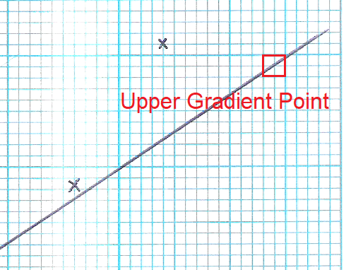
6. Find the lower and upper gradient points of the line of 'best fit'
- These points will greatly assist in finding the gradient of the line of 'best fit'.
- These points are found where the line of 'best fit' cuts an intersection of a horizontal and vertical line as shown in Figure 6 and 7. The further apart these points are on the line the more accurate your gradient value will be.
- These points should never be points plotted points from the table. Always take the lower and upper gradient points from the line of 'best fit'.
- The lower gradient point is found near the origin and the upper gradient point is found near the end of the line of 'best fit'.
 | ||
Figure 6
|

 |
| Figure 8 |
7. Calculate the gradient with units.
Comments:- The gradient is calculated using the formula: gradient = (change in y) ÷ (change in x)
- In this example, the gradient quantity is acceleration.

Example 2
An experiment on a spring which obeys Hooke's Law produces the following results of Load and Length.
Table 2 showing the load and
length of a spring under an experiment.
Load / N
|
4.0
|
8.0
|
12.0
|
16.0
|
20.0
|
24.0
|
28.0
|
32.0
|
Length / mm
|
18.4
|
20.5
|
22.4
|
24.3
|
26.4
|
28.5
|
31.3
|
36.4
|
- Plot a graph of Length against Load.
- Calculate the gradient of the graph, including its unit.
Solution Steps:
1. Draw your x and y axes.
 |
| Figure 9 |
2. Head your graph and Label the axes.
 |
| Figure 10 |
3. Calibrate your x and y axes and place your Scale.
Comments:
- The best suited scale of the x-axis is 5.0 N for every 2 cm because it accommodates the range of values for Load and it spans for the entire axis.
- The best suited scale of the y-axis is 4.0 mm for every 2 cm because it accommodates the range of values for Length and with a smallest division of 0.4 mm, I am able to locate precise measurements, such as 18.4 mm, 22.4 mm, 26.4 mm, etc.
- The smallest division is value by which each axis is incremented by. It is calculated using the formula: Smallest Division = Calibration ÷ Number of Lines
The smallest division on the x-axis is 0.5 N and on the y-axis is 0.4 mm.
Did you find the smallest division for example 1?
 |
| Figure 11 |
4. Plot the points using ⊙ or a small 🗙
 |
| Figure 12 |
5. Draw the line of 'best fit'.
Comments:
- Notice the line of 'best fit' meets the y-axis above the origin as shown in Figure 13. Recall, the line of 'best fit' is a straight line which passes through most of the points but not necessarily all the points.
- Recall also, the spring obeys Hooke's Law, which states that the force applied to a spring is directly proportional to its extension. If the spring is extended beyond this portion of proportionality then the straight line would begin to curve as shown by the last plotted point.
 |
| Figure 13 |
6. Find the lower and upper gradient points of the line of 'best fit'
 |
| Figure 14 |
 |
| Figure 15 |
 |
| Figure 16 |
7. Calculate the gradient with units.
Comments:
- The gradient quantity for this graph is the reciprocal of the spring's constant of proportionality.
- The gradient was calculated with its unit and was given to three significant figures


0 Comments